Big Data Guy

Mapping Acoustic Evolution: A Data Dive into 1969 vs. 2019 Billboard Hot 100 Hits

The Big Question 🤔

If you’ve ever asked your parents about their taste in music, how would you describe the differences between their preferences and your own? What about your grandparents? This analysis examines acoustic and other data from hit songs from 1969 and 2019 to answer the question: How have musical tastes and trends in the music industry evolved over the decades?

Prerequisites: This post assumes beginner to intermediate-level experience in Python, as well as a basic understanding of web scraping and APIs. We will avoid delving into the technical specifics of certain Python functionalities to provide a more generalized tutorial. The complete code is available in this GitHub repo and in this Google Colab notebook.

Learning Goals 🎯

• Understand the basics of API usage, particularly with the MusicBrainz and AcousticBrainz APIs.
• Learn how the acoustic features of popular songs have changed since 1969.

What are people listening to? 🎧

The Billboard Hot 100 is a weekly chart that ranks the most popular songs in the United States. It has been a staple of the music industry since its inception in 1958. By analyzing certain features of songs that have topped the Billboard Hot 100 in 1969 and 2019, we can gain insight into how musical tastes have evolved over the years. To conduct our analysis, we first need data. We will use this GitHub repository, which contains a dataset of historical Billboard Hot 100 tracks from 1958 onward.

After loading the dataset, we filter it to include only songs from 1969 and 2019, saving each dataframe as a CSV file for later use. We do not remove duplicates, as we assume that a song’s repeated appearance on the Billboard Hot 100 indicates its popularity and lasting appeal.

Let’s compare the first two songs in each dataframe:

print(f"2019: {billboard_df_2019['song'][0]} by {billboard_df_2019['artist'][0]}\n"
      f"1969: {billboard_df_1969['song'][0]} by {billboard_df_1969['artist'][0]}")

output:

2019: Thank U, Next by Ariana Grande

1969: I Heard It Through The Grapevine by Marvin Gaye

Ah, yes. One song about exes and another about rumors. Truly, the Billboard Hot 100 has always been a melting pot of gossip-related themes!

Using the MusicBrainz API 🧠

Now that we have our songs, we need to uncover their acoustic features. We will use AcousticBrainz, which works best with a specific song ID (called an MBID). First, we need to extract each song’s MBID. Think of an MBID as a unique fingerprint for each song. With this fingerprint, we can find specific details about the song. To get these IDs, we will use MusicBrainz. To start using the API, we need the base URL, a ‘query’ (how we will look up each song), and our ‘User-Agent’ (identifying ourselves to the website). Website owners like to know who is using their data.

Note: ⚠️ Always review API documentation. Ethical data collection is key for any use case. You can find the MusicBrainz API documentation here. Each API has its own specific syntax, requirements, and limitations. It is crucial to adhere to the guidelines in the API documentation when collecting data, as failure to do so may result in access revocation or even legal action. Furthermore, respecting these guidelines demonstrates good citizenship within the developer community. The data collected for this project was gathered ethically, adhering to the API documentation and respecting rate limits. The process was streamlined by carefully following the syntax outlined in the API rules. ⚠️

First, we define a function to extract the MBID of any song:

def get_recording_mbid(song, artist):
    # define our base url
    url = "https://musicbrainz.org/ws/2/recording"

    # query is what will be searched
    query = f'"{song}" by "{artist}"'

    params = {
        'query': query,
        'fmt': 'json',
        'limit': 1 # limit 1 indicates that we only want the first entry
        }

    headers = {
        # here you put the name of your application/purpose of API usage
        # as well as your email to identify who you are
        'User-Agent': 'DataAnalysis/1.0 (youremail@exampledomain.com)'
        }
    
    try:
        response = requests.get( #get the data!!!
            url,
            params=params,
            headers=headers
            )
        # here we normalize our json output, selecting only the recording part of the multi-nested list, 
        # selecting the first element of the first list and only the 'id', this will give us the MBID
        return pd.json_normalize(response.json())['recordings'][0][0]['id']
    
    except: # in the case of an error, put a null value in the cell
        return None

Let’s see how it works! get_recording_mbid(billboard_df_2019[‘song’], billboard_df_2019[‘artist’]) gives us the MBID for “Thank U, Next” and outputs 274b3a7b-64bd-4af3-9af9-dd41277ddc17.

With the function working, we can create a for loop to extract the MBID of every song in both dataframes.

Note: The MusicBrainz API has a rate limit of 10 requests per 10 seconds. Our code uses a sleep timer of 1.5 seconds to be safe. Remember not to exceed the rate limit, or you will be temporarily (or even permanently) banned.

Extracting Song Features 🎵

Finally, we can extract the acoustic features of each song using the AcousticBrainz API. We define a function called get_song_features. The most important part is that we take an MBID as input and fetch the features based on their level using separate links. Low-level features are more objective, such as key signature and BPM, while high-level features are more subjective, such as danceability, energy, and loudness. These features are computed by an algorithm that can be found here. Check the details for all AcousticBrainz features and API documentation here.

Let’s check out the features for Mariah Carey’s ‘All I Want For Christmas Is You’:

get_song_features(billboard_df_2019['mbid'][2])
output: {'danceability': 'danceable', 'genre': 'pop',
'gender': 'female', 'mood': 'not_aggressive',
'instrumental': 'voice', 'bpm': 150.164459229,
'key': 'G', 'loudness': 0.871298909187,
'mood_happy': 'happy'}

It seems fairly accurate, although I don’t remember the song being particularly loud.

After defining the function, we need to loop through each dataframe to retrieve the features of each song. Essentially, we loop through the dataframe, running the get_song_features function to extract each row’s features and assign them to the corresponding column. An optimized version of this loop is included in the code.

Now we can save the results and analyze the data!

Note: The complete data retrieved from running this code is in the GitHub repository.

The Big Picture 🖼️

First, let’s look at what we have:

print(f"Number of songs from 1969: {len(billboard_df_1969)}")
print(f"Number of songs from 2019: {len(billboard_df_2019)}")

output:

Number of songs from 1969: 2248

Number of songs from 2019: 2547

Not too shabby; we were able to retrieve the features for about half of the songs.

Are We Going Deaf? 👂

Have your parents ever told you that the music you listen to is too loud? Let’s compare and see if we are really damaging our eardrums.

print(f"Mean loudness coefficient in 1969: {billboard_df_1969['loudness'].mean()}")
print(f"Mean loudness coefficient in 2019: {billboard_df_2019['loudness'].mean()}")

output:

Mean loudness coefficient in 1969: 0.7608138030109645

Mean loudness coefficient in 2019: 0.8266435674148748

Well, it certainly has increased. I’m not quite sure what this means for our ears, however. More on the loudness feature’s interpretability here.

From Mood Swings to Who’s Causing Them 💔

We extracted a feature called mood_happy. This tells us whether the algorithm classified the song as ‘happy’ or ‘not happy’. Plotting the proportion of moods for both years gives us the following bar plot:

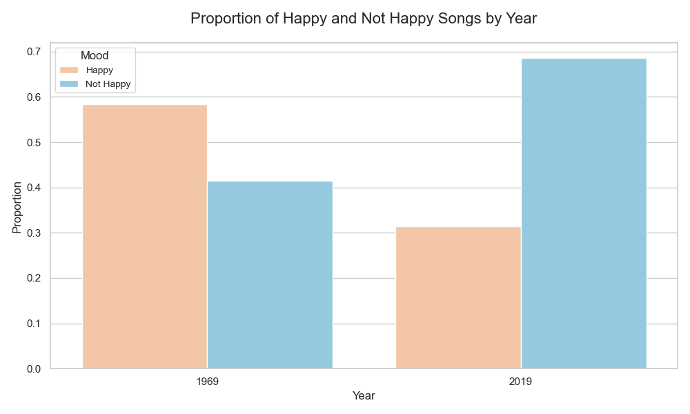
The proportion of happy songs has decreased significantly. I guess heartbreak wasn’t trending in 1969 as much as it is now.

Let’s look at the proportion of artists recognized as ‘male’ or ‘female’:

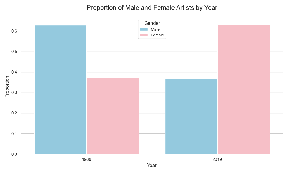
Cool! These would be interesting topics to explore further.

One-Hit Wonders: Then vs. Now 🌟

We conclude by looking at the longevity of songs on the Billboard Hot 100. We are taking unique songs that have been in the #1-5 position and looking at the maximum number of weeks they were on the chart.

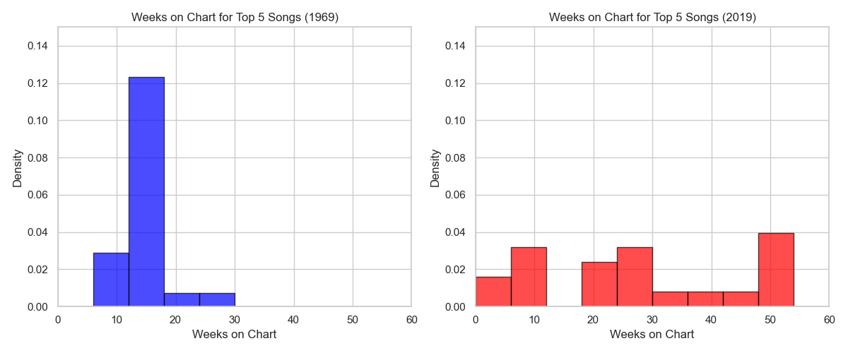
It seems songs last longer on the Billboard Hot 100 these days. I imagine several factors contribute to this.

What’s Next? 🚀

Before concluding, here are some ideas to spark curiosity:

• How do certain features (mood, danceability, etc.) differ between months in each year?
• What similarities between genres are seen between the two years? How do they differ?
• How does the number of unique artists in the top 5 compare between 1969 and 2019? Is there more diversity in recent years?
• What is the relationship between a song’s peak position and its total weeks on the chart?

Conclusion and Final Thoughts 💭

In this post, we learned the basics of API usage and how hit songs have changed over the decades. Now, go experiment with the APIs we reviewed or others you find!

For other resources, see below:

• Discover how to use the Essentia open-source library for more audio analysis in Python here.
• Learn advanced EDA with Seaborn Tutorials.

Found this helpful? Share it with a friend or tweet about it!

Link to GitHub repository